Reading a wildlife spectrogram

Orient the three dimensions

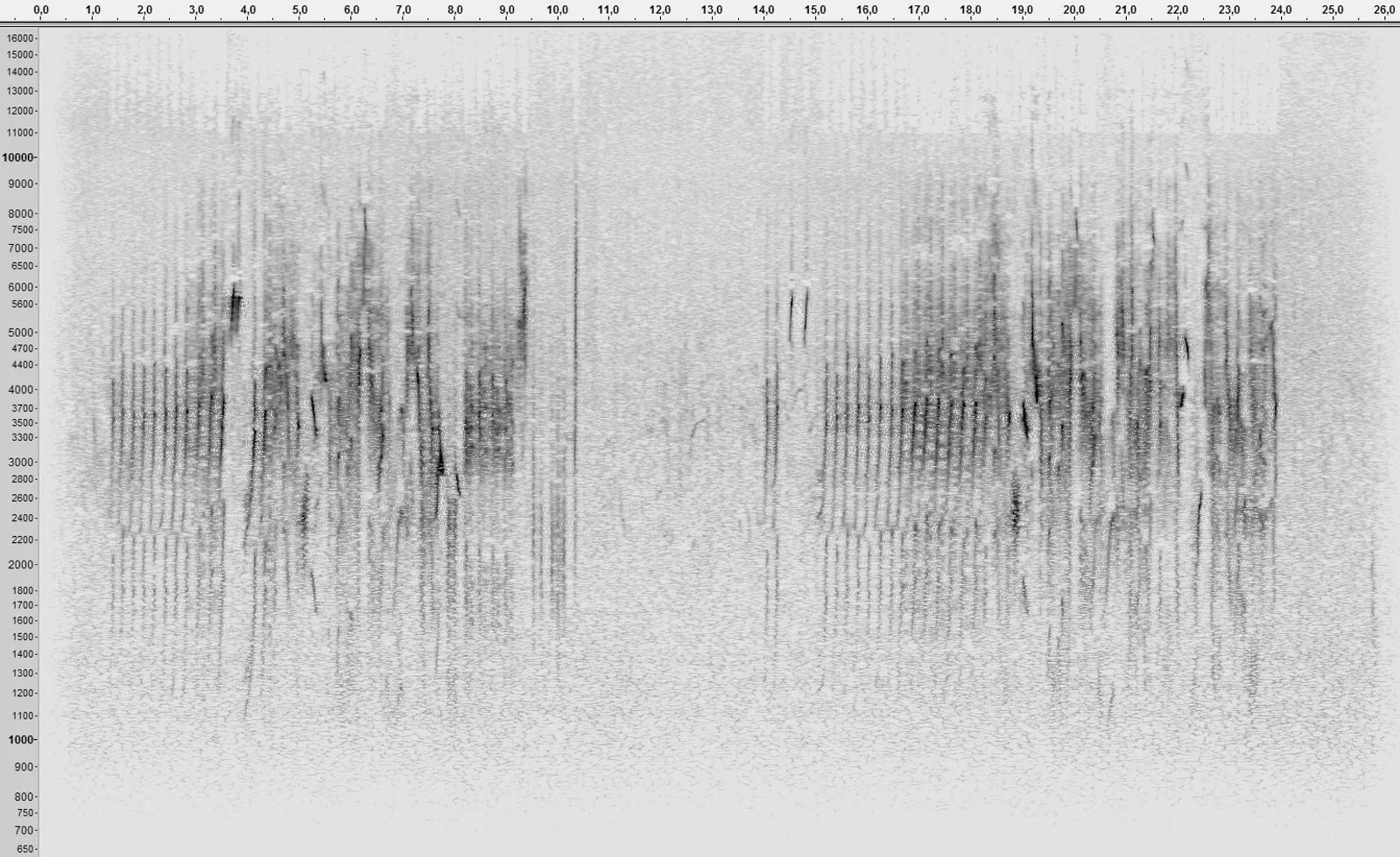
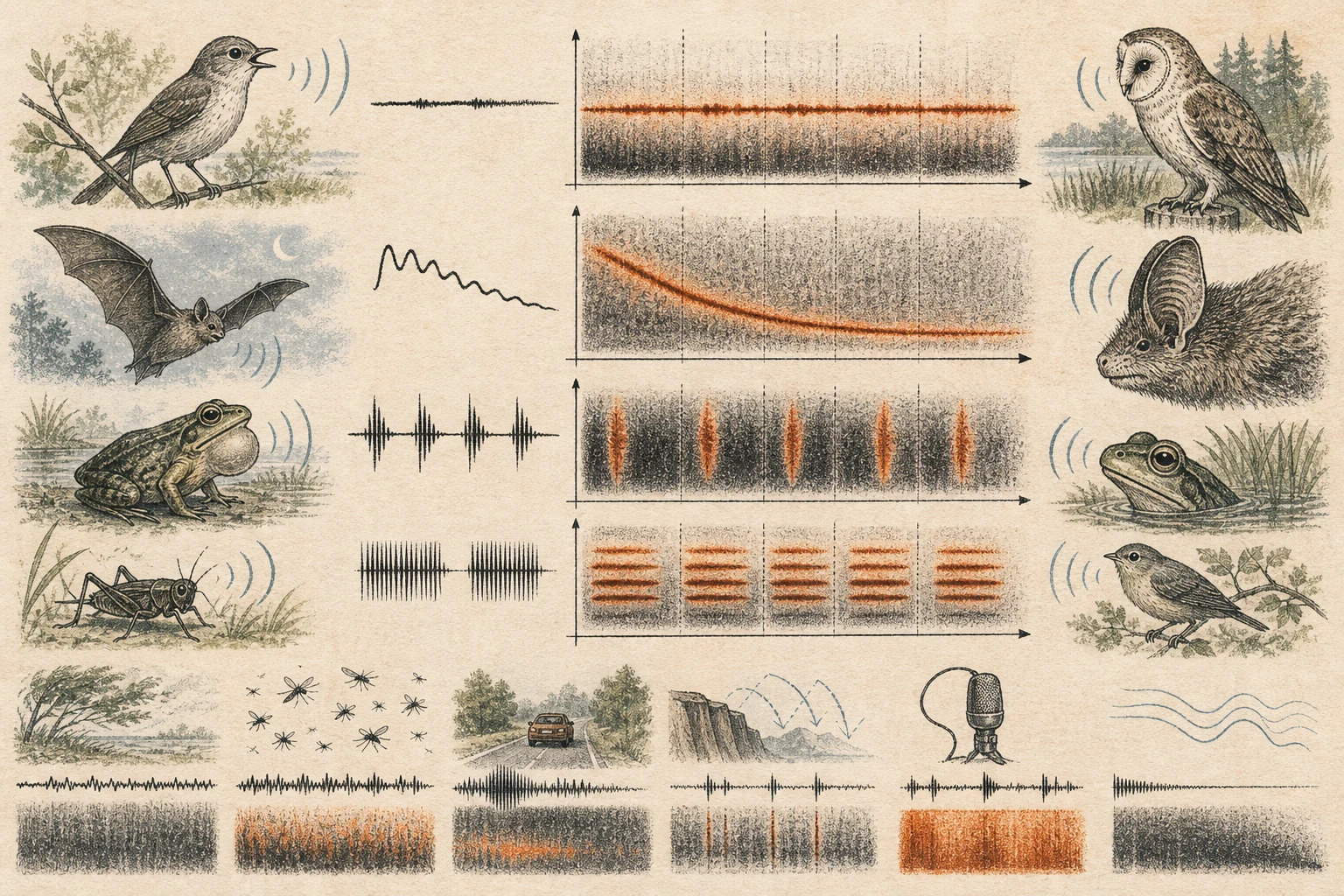
When you open a field recording of a dawn warbler, calling treefrog, or passing bat in acoustic software, the spectrogram plots three variables at once: time runs from left to right along the horizontal axis, frequency climbs from low bass to high treble along the vertical axis, and pixel darkness or color brightness represents relative acoustic energy inside each time-frequency cell. Note that visual intensity shows energy at the microphone rather than how loud a sound feels to human ears, which vary in sensitivity across pitches. Always inspect the printed axis numbers before comparing two screenshots, because stretching the time scale, cropping the kilohertz ceiling, or boosting display gain can make identical vocalizations look completely different. [1][2]

• Check the horizontal seconds scale and vertical kilohertz range before comparing two spectrogram images.
• Read darker or brighter color values as relative acoustic energy at the microphone, not standardized loudness.
• Keep time and frequency scales uniform when assembling comparison plates for similar-sounding species.

Translate shapes back into sound

With a little practice, visual marks on the screen map directly onto what you hear through headphones in the field. A flat horizontal band marks a steady whistle or pure tone; a steep upward or downward arc shows a frequency-modulated sweep; a tight picket fence of vertical lines reveals rapid broadband clicks, bill snaps, or insect stridulation. When several parallel ribbons stack at whole-number multiples of the lowest band, you are usually looking at harmonics generated by a single vocal tract rather than a chorus of separate callers. Measure note duration, inter-note pauses, peak energy frequency, and phrase rhythm, then replay the audio while watching the cursor cross each trace. [1][3]

• Match flat traces to steady whistles, sloped curves to pitch sweeps, and sharp vertical bars to clicks or percussive taps.
• Recognize evenly spaced parallel bands stacked above a fundamental frequency as harmonics from one vocalizing animal.
• Measure note length, pause intervals, and peak frequency directly from the axes rather than relying on visual impression.

The window changes what you see

A spectrogram is not a raw photograph of sound; software computes it by slicing the waveform into overlapping analysis windows and running a Fourier transform on each slice. Because of the time-frequency uncertainty principle, window length forces a direct trade-off. Choosing a long window with a large FFT size separates closely spaced frequencies and harmonic stacks cleanly, but smears rapid trills along the time axis. Choosing a short window sharpens the exact onset and gap of fast clicks or pulses, yet thickens horizontal pitch lines into blurry ribbons. Low-frequency rumbles and rapid high-pitched trills often benefit from different display settings, so never attribute differences between two images to the animal until their window parameters match. [2][4]

• Increase window length (FFT size) when you need to resolve fine pitch contours or closely spaced harmonic bands.
• Shorten window length when measuring millisecond pulse rates in insect stridulation, woodpeckers, or rapid trills.
• Record the FFT size, window function, and overlap percentage whenever you export a spectrogram for comparison.

Treat the display as measured evidence

Field recordings carry the signature of the environment and equipment alongside the target animal. Wind buffeting the microphone floods the bottom of the plot with dark low-frequency rumble; forest reverberation trails blurry tails behind sharp notes; clipping creates artificial harmonic ghosts; and aggressive high-pass filters or lossy file compression can slice away real syllables. Furthermore, no recording can faithfully represent frequencies above half its digital sampling rate (the Nyquist limit), and distant quiet notes often vanish into the background noise floor. Pair spectrogram measurements with date, locality, habitat, behavior notes, and careful listening before proposing an identification. [3][4]

• Watch for reverberation tails in woodland recordings that can make crisp notes look longer and more slurred than they are.
• Verify that your recorder's sample rate is at least double the highest frequency produced by your target group.
• Combine spectrogram measurements with field context, range, and direct listening rather than matching one shape in isolation.

Related guides

• Recording wildlife sounds for identification
• Why birds sing
• How bat echolocation works
• How bird-song ID apps work